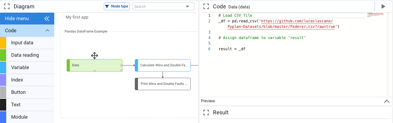
One of the distinctive aspects of Pyplan is the way in which the code is organized through a hierarchical influence diagram, where each node represents some stage in the loading or processing of information.

Nodes are repositories of portions of code that can be entered directly by the user or generated automatically by a Pyplan wizard when parameterizing or manipulating interfaces developed for this purpose.
The diagram is constructed by dragging the different node types onto the diagram sheet. The node window is expanded by clicking on this icon |expand| that appears in the upper left corner of the diagram.
Arrows indicating the relationship between nodes are automatically generated when a variable is referenced as a source of input data for a subsequent process.
The nodes have different colors that help to understand their function within the diagram.
¶ No-code
Pyplan is a platform designed for users without programming skills to build and share Data Analytics and Planning applications.
The construction of an application requires as a first step the input of data, which can be manual or through the reading of an external data source.
¶ Manual Data Input
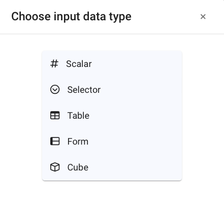
The manual data input is constructed by dragging a node of the type:

This type of node, once a title has been defined, opens a wizard that allows you to define the type of manual data to be entered.
¶ Scalar Entry
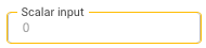
This is the input used to enter a single parameter. Once the node title has been defined, it is represented in the diagram as follows:
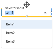
¶ Selector Input
It is used to enter the different choice alternatives that will be presented in a drop-down selector. Once created, it appears as follows in the diagram:
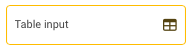
¶ Table Input
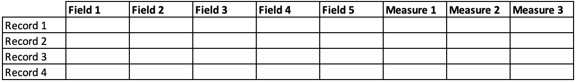
It is used to enter multiple parameters that are organized in a table structure, where each column represents an attribute and in each row a record is entered. After entering a title for the node, a wizard opens that allows you to define the fields that will constitute the data table and the type of data that will be entered.
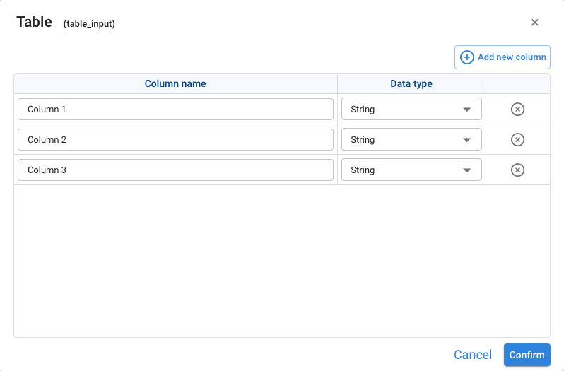
Once created, it will appear as follows in the diagram:
Selecting the table node, and then double-clicking on it, opens the full-screen table for data entry.
Table Storage. The data loaded here are stored in an object called Pandas Dataframe. Pyplan interprets this type of objects natively, allowing their manipulation and visualization in table and graphic form.
¶ Form Input
The form is the most powerful and versatile manual data entry tool since it allows combining data entry columns together with calculated columns that serve as a reference or guide for the data being entered. For example, if we are creating a tool to enter data for a sales budget, it may be helpful for the person who is going to enter that data to have the previous year’s sales as a reference. The form, unlike the Table, is stored in a database, thus allowing multiple users to enter data simultaneously.
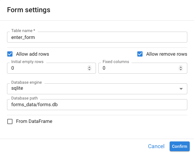
When dragging a data entry node, and after having chosen Form as input element, the following wizard for its creation is displayed:
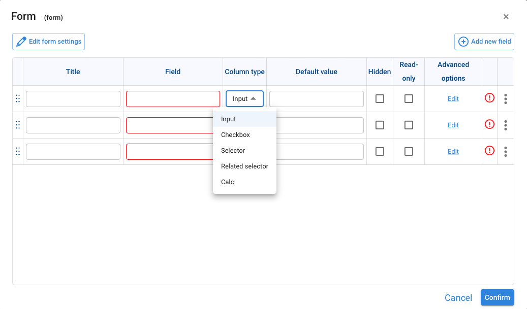
By defining a title for each input field, a field name suggestion is generated, then the column type according to the options shown in the drop-down box.
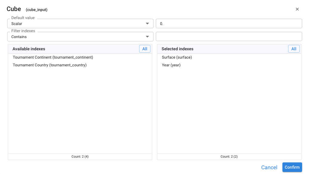
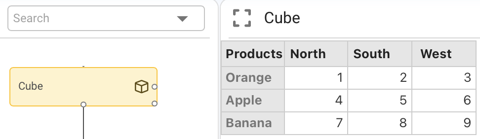
¶ Cube input
A data cube is a particular input object that allows the input of a single parameter for all combinations of cube dimensions. This is why for its definition it is necessary to indicate which are the dimensions of the input data cube. Its use is indicated when you want to emphasize the data entry in all elements of the opening dimensions.
¶ Data source reading
Another way to enter data into Pyplan is by connecting to external data sources, which are read when the corresponding code is executed.

For this purpose, drag a node named data reading that will display, after defining its title, a dialog box like the following one:
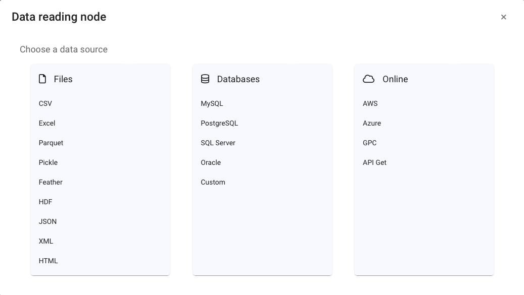
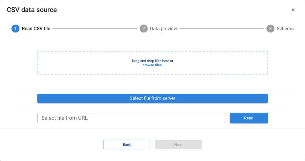
The most frequently used options (csv, Excel) also have a specific wizard that allows you to configure all the reading parameters.
Other less frequently used options are initialized with the base code which, after completing the necessary parameters, allow the corresponding data reading.
¶ Data Manipulation and Operations

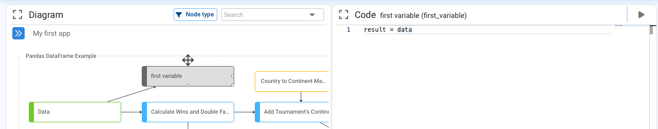
Once the data entries have been generated, the next step is their analysis and processing, for this purpose the variable type nodes are used. This type of node is the most general of all and allows any type of coding to be included in its definition. When dragging and dropping a “Variable” node, we will be asked to define its title and then we will obtain a node with a definition like the following one:
result = 0
To link this new node with another one that is its data source, we can write the node’s identifier (Id) in its definition or once positioned where we want to insert the call to another node, pressing the <Alt> key we click on the node to which we want to link it, this will bring the Id of that node to the definition.
Accepting the changes we will see that an arrow appears indicating the link between nodes and the color of the variable node changes to “Gray” to indicate that this process has no other output beyond the node itself.
The Variable type node allows writing Python code freely in its definition. However, Pyplan provides a series of wizards that help to perform data transformation operations through the use of interfaces prepared for this purpose.
These wizards depend on the data structure we are working with (object), this is why we need to evaluate the node first so Pyplan can determine the wizards it will present us to work with.
These wizards are identified as “Wizards” and are displayed once the node has been executed, by clicking on the icon shown in the following figure:
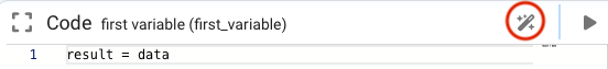
When using these wizards, you will be able to observe how the node definition code changes with the appropriate instructions to generate the desired process. This procedure, equivalent to recording Macros in a spreadsheet, allows the user who does not know the Python language to be introduced to its functions and syntax.
¶ Indexes
The indices or dimensions are the way in which the data is structured. That is, they are the row and column headings of a table that describe what the value we see at their intersection is about. Examples of indexes are the list of products, regions, time periods, etc. They serve to characterize the data or facts with which we operate.
In Pyplan, the indexes are generated by dragging a specific node type for this purpose identified as
After entering a title for the Index, a wizard is displayed to define the elements of the index.
¶ List
Allows manual entry of the index elements. It is also possible to copy them from a table and paste them indicating their first position. The data range will be extended if it is greater than the number of elements displayed.
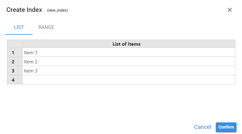
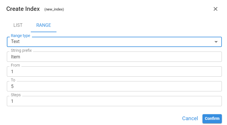
¶ Range
Allows to generate the index automatically by defining the parameters of a range. This range can be of type text, number or date

¶ Hierarchy of indexes
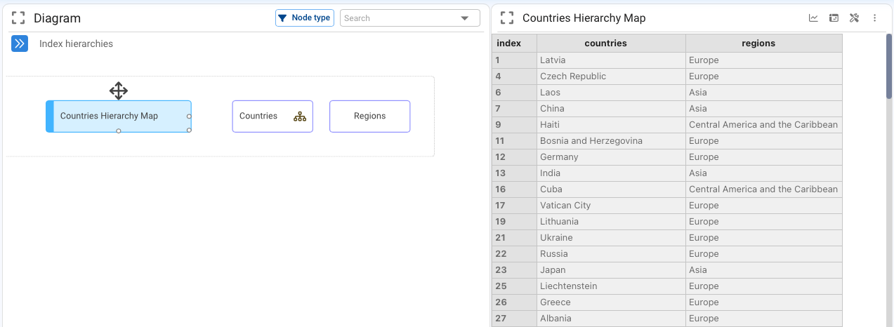
Indexes can also have hierarchies, i.e. higher levels of aggregation. For example, the natural hierarchy of a Country index is Region or Continent, or that of a Month index is Quarter, Semester or Year.
The correspondence between an index and its upper hierarchy is established through a table where for each element of the lower hierarchy its corresponding element in the upper hierarchy is indicated. The following image illustrates the case for an index “Countries” and its upper hierarchy “Regions”
By right-clicking on the lower hierarchy index, its properties indicate which table contains the correspondence relation with the upper hierarchy, following the example:
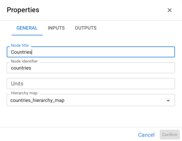
Any index containing a hierarchical relationship is identified with an icon inside the node as shown in the following image in the Countries node
¶ Organization of the diagram
The diagram or “workflow “ is the way the code is organized in Pyplan. A general convention to aid readability is to keep the direction of the arrows / flow of information from left to right and from top to bottom. In addition to headings to summarize the process or information housed in a node, it is possible to include text boxes to help interpret a set of nodes.
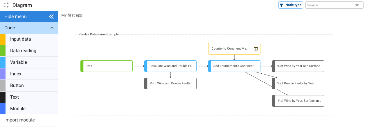
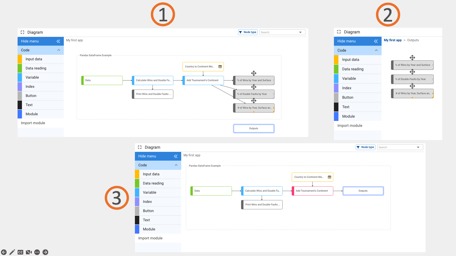
As a general rule it is desirable not to have more than 20 nodes in a diagram. Whenever this happens it is recommended to use “Modules” to group nodes whose process share a specific purpose and therefore can be grouped together.
In the above diagram we could create a module called “Outputs” (1) that groups the 3 output nodes. And then cut (2) and paste (3) the output nodes into the new module.
These 3 steps are described in the following image:
¶ Node coloration
Nodes are automatically colored to facilitate the understanding of their purpose and function.
All nodes keep their original color, which is the one displayed in the menu from where they are dragged, except for the Variable node. This node can take three colors according to its function:
light blue: when it is part of a calculation process in the diagram containing it
gray: when the node in question has no outputs
red: when the node’s outputs are outside the module that contains it
¶ Node execution
A node can have two states: Not Calculated or Calculated.
When opening an application all the nodes are pending execution, until some command indicates it. When a node is commanded to compute (execute), Pyplan recursively goes through the entire influence diagram asking if the nodes that feed the node to be executed are computed, if not, it goes one step back in the computation process asking the same question.
Once the application boundary or the boundary of the computed nodes is reached, it starts to compute downstream in order to finally present the result of the queried node.
This process guarantees that the result of a node when calculated is always the same and that its value does not depend on the execution sequence of the preceding nodes.
On the other hand, this mechanism provides a lot of computational efficiency since changing any intermediate variable in the calculation guarantees that only those nodes whose value has been affected by the change in the mentioned variable are recalculated.
The status Calculated / Not calculated can be inspected when selecting a node. In the result view it will show the output of the node if it is calculated and otherwise a message indicating that the node is not calculated.
¶ Data structures supported
Pyplan natively interprets some data structures such as Tables and Cubes coming from the most widespread Python libraries (Pandas, Nump, etc.).
Data tables are the typical structure of a database, with attributes defined by columns, where each row corresponds to a record.
Data cubes can have any number of dimensions. These dimensions in turn can be nominated or undefined.
Most commonly used data structures
¶ Data tables
A table is similar to a database table, i.e. it is a data structure where each column represents an attribute or measure and where each row corresponds to a particular record of those attributes or measures.
|br|The data tables in Pyplan correspond to the Dataframe object of the Pandas library, one of the most used libraries in Data Science. Some basic functionalities of operations with Dataframes are provided by the Pyplan wizards. There are however many other operations that can be performed through Python coding using the Pandas library.
Pandas Quick Introduction
A quick introductory guide to Pandas functionalities can be found here.
¶ Assisted operations with Tables
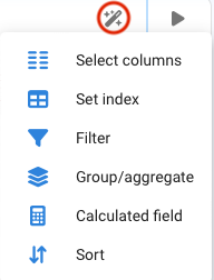
A node that when evaluated returns a Table (DataFrame) as a result will present the following options as assistants:
Continuing with the example, if we create a variable “first variable”, we change its definition by linking it to the node data such that:
result = data
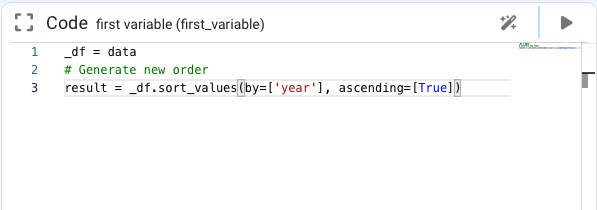
after executing this node to allow Pyplan to identify the resulting object, we deploy the wizards and choose sort “by Year”
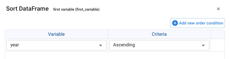
We will see that the result is the sorting by year of the table and its final code is defined as follows:
The user could continue to interact with the data object and analyze the changes it causes in the node definition and thus learn the Python language.
¶ Data cubes
The data cube is also an object natively supported by Pyplan. The object used is the DataArray from the XArray library. A named data cube is a data structure containing a values indexed by n-identified dimensions. These dimensions in Pyplan are called Indexes and are identified by this type of node
in the diagram.
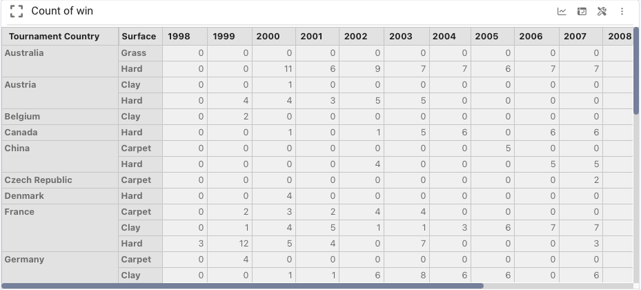
For example, we could think of a “Count of Win” data cube indexed by the dimensions [Tournament Country, Surface, Year]
This cube, following the example developed so far, would be:
Data cubes are created by transformation of tables (Dataframes) into data cubes, by direct inputs (Input Table), or by operations between cubes.
¶ Creating a Cube from a Data Table
Right-clicking on a node that is evaluated as a data table displays the following menu:
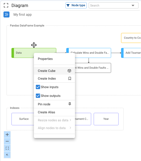
Clicking on the “Create Cube “ option displays the following dialog box:
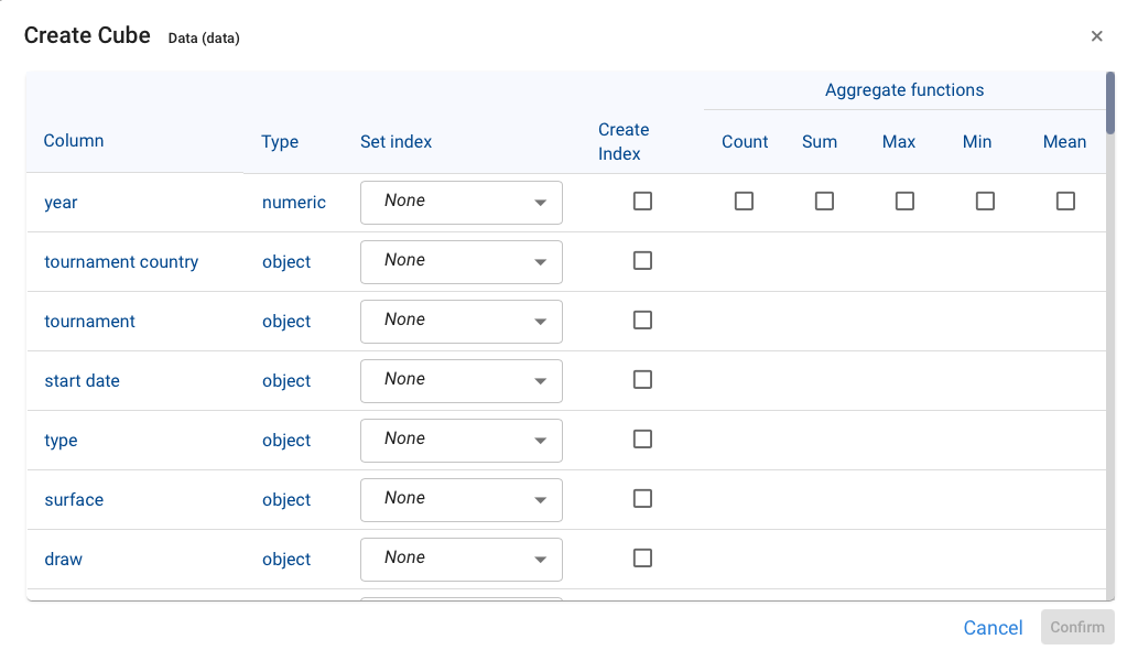
It lists all the columns of the dataframe, the type of data, the index (if it exists) that will collect the values of that column, the option to create an index in case it does not exist and finally the aggregation function that will be used to group the value of the fact or variable to be represented.
To create a data cube in Pyplan it is necessary to have, in advance, the dimensions (Index) that characterize the data cube. It is for this reason that the wizard offers us to create the indexes based on the column data in case it does not exist.
¶ Operations with data cubes
As with Table type objects, Pyplan provides wizards to operate with Data Cubes, which are automatically deployed in the same place, when the resulting object is a Data Cube of type XArray.
Additionally, unlike Tables, Data Cubes allow mathematical operations between them that result in new Cubes. It is important to understand how these operations between data cubes work in order to build the desired calculation process.
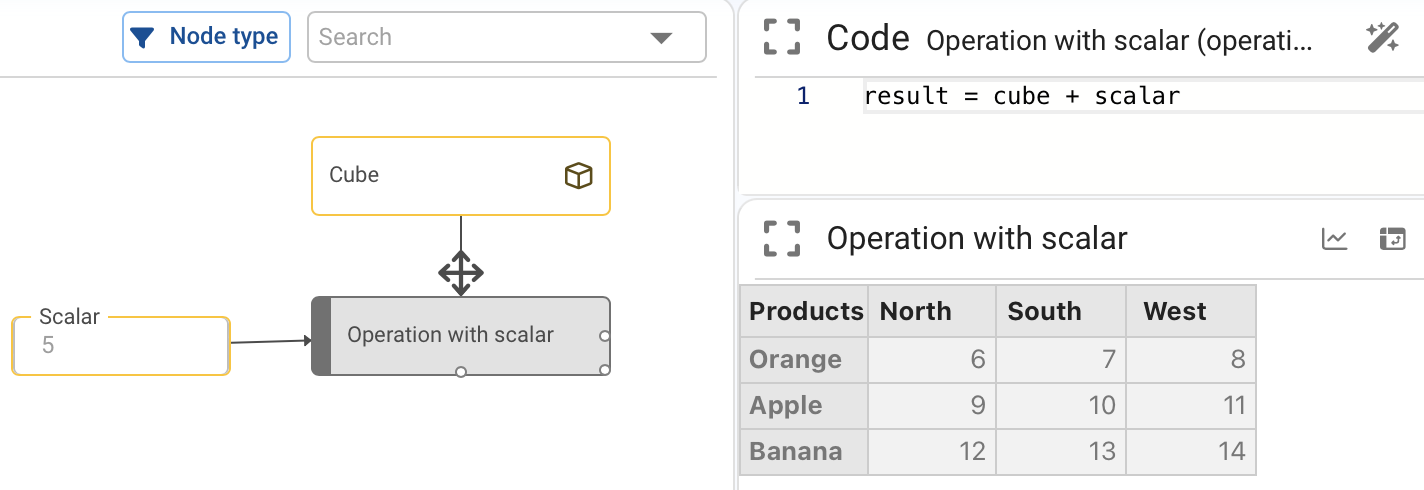
¶ Operations between a scalar and a cube
When adding, subtracting, multiplying or any other mathematical operation on a data cube, it is performed between the scalar and each element of the data cube.
The following image shows the definition of the node it establishes:
result = cube + scalar
The value of the scalar, 5 in this case, is added to each element of the original cube giving as a result:
¶ Operations between two cubes of equal dimensions
In case the cubes have the same dimensions, the indicated operation is performed between the elements of the same cells of both cubes
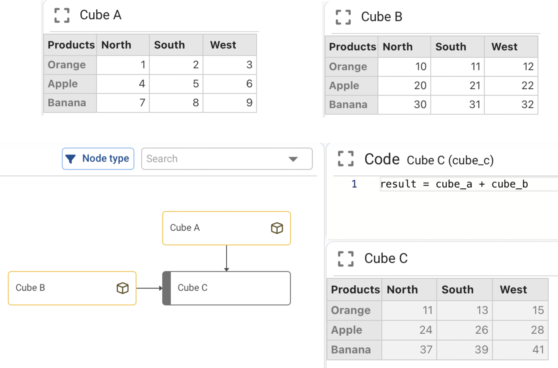
In this case we can see how the first cell of Cube C is the result of the sum of the first cell of Cube A plus the first cell of Cube B.
¶ Operations between two cubes of different dimensions
When operating with cubes of different dimensions, the missing dimension in one of the cubes operates scalarly on the other cube. An example allows to better explain this way of operating:
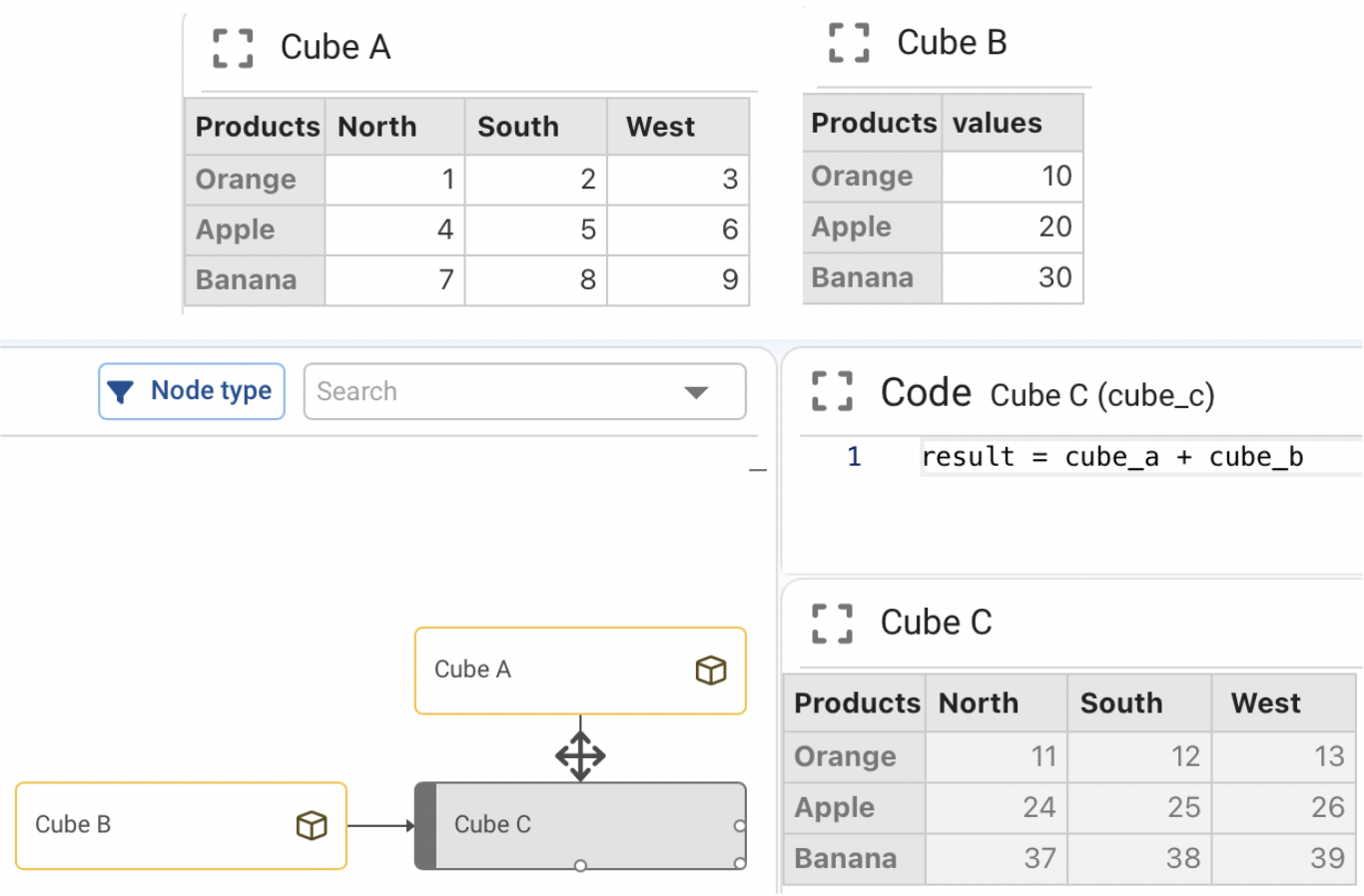
In the example above you can see how Cube B, which does not have the dimension Region, is used in a scalar way with respect to this dimension when operating with Cube A.
The complete list of operations with Cubes can be found in the ``documentation of the XArray library. <https://docs.xarray.dev/en/stable/user-guide/computation.html>`_
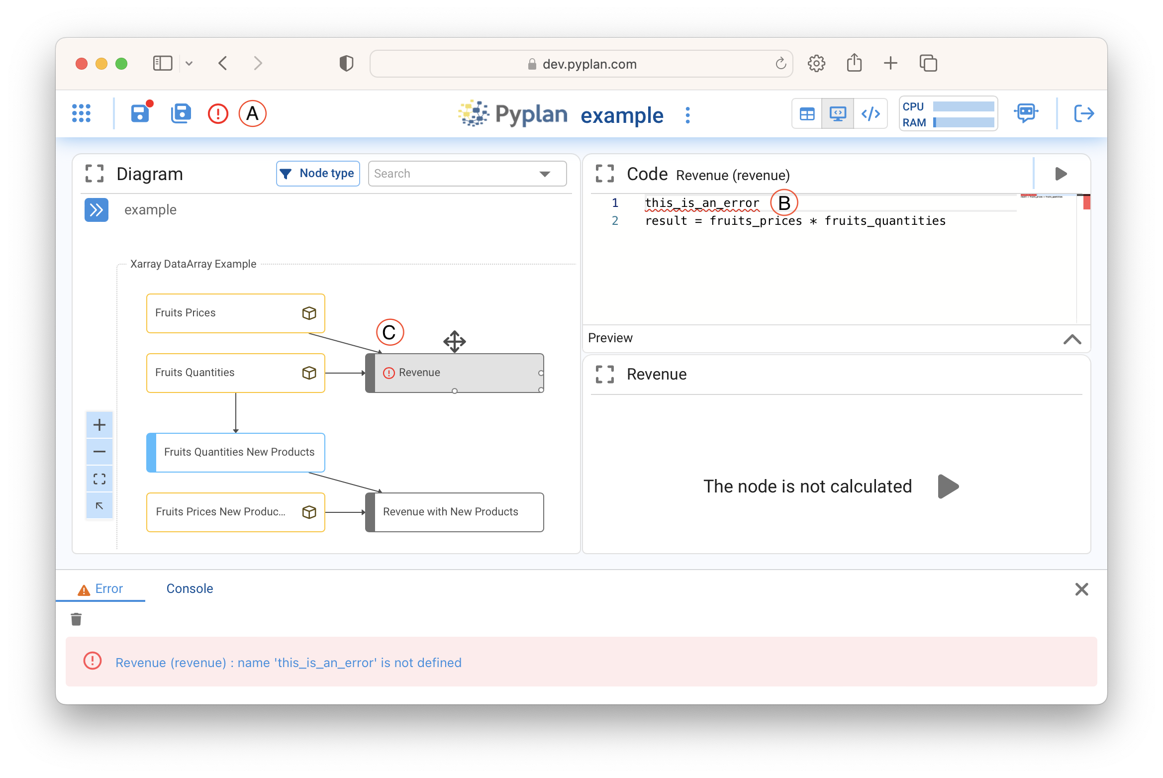
¶ Error console
When an error occurs in the execution of the code, it is indicated with a warning sign (A) as shown in the following image. Clicking on this indicator displays the error console at the bottom. In addition, the line with error (B) is underlined in red inside the code. The node containing the error (C) is also marked.