No Code
Pyplan is a platform designed so that users without programming skills can build and share Data Analytics and Planning applications. Building an application always starts with data input, which can be done manually or by reading from an external data source.
Manual Data Input
We create manual inputs by dragging an Input data node onto the influence diagram.
![]()
After giving the node a title, Pyplan opens a wizard where we choose and configure the type of manual input we want to use.
Scalar Input
A Scalar Input is used to enter a single parameter (for example, a discount rate, an exchange rate, or a growth assumption). Once we define the node title, the Scalar Input appears in the diagram as a simple node representing that value.
![]()
Selector Input
A Selector Input is used to define a list of alternatives that will be shown in a drop‑down selector (for example, scenario, region, product line). The node provides a selectable list that can be used by other nodes in the model.

Form Input
The Form Input is the most powerful and flexible manual data‑entry option. It lets us combine input columns (where users type values) with calculated columns that act as references or guides. Form data is stored in a database, enabling multiple users to enter or update data simultaneously.
When we drag an Input data node and choose Form as the input type, Pyplan opens a configuration wizard where we define a title for each input field and choose the column type (number, text, date, etc.).
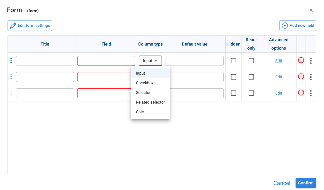
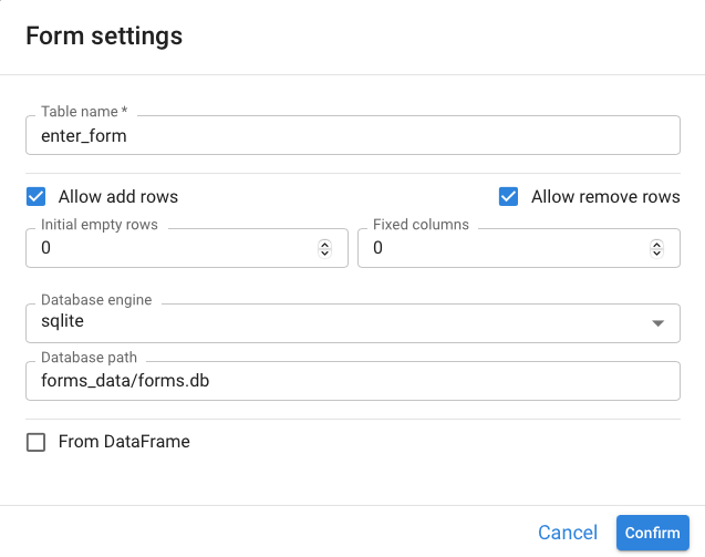
Pyplan then opens the Form settings window to configure how the form will behave and how its data will be stored:
| Setting | Description |
|---|---|
| Table name | Name of the table in the database (must be unique). |
| Allow add rows | When enabled, users can add new rows in the form. |
| Allow remove rows | When enabled, users can delete existing rows from the form. |
| Initial empty rows | Number of blank rows created when the form is first opened. |
| Fixed columns | Number of columns that cannot be removed by end users. |
| Database engine | Storage engine used for the form data (e.g., sqlite, PostgreSQL). |
| Database path | Physical path or connection string to the database. |
| From DataFrame | When checked, the form can be initialized from an existing DataFrame's structure. |
Cube Input
A Cube input node lets us enter a single value for every combination of a set of dimensions (indexes). When we create or edit a Cube input, Pyplan opens the Cube settings dialog:
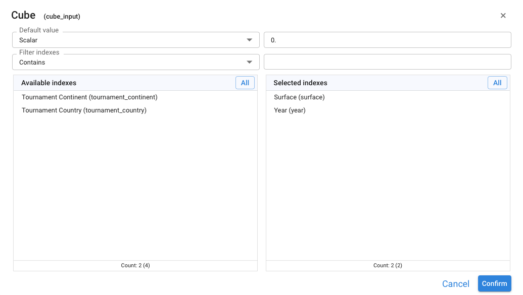
The dialog has four main parts:
- Default value — Defines the value used initially for all cells (scalar literal or from another app node).
- Filter indexes — Optional filter to help search indexes when there are many.
- Available indexes — Lists all Index nodes that can be used as dimensions of the cube.
- Selected indexes — Shows the indexes that will define the dimensions of this Cube input.
Data Source Reading
Another way to load data is by connecting to external data sources, which are read when the node's code is executed.
![]()
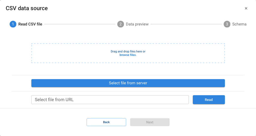
To do this, drag a Data reading node onto the diagram. After defining its title, Pyplan opens a dialog where we choose the source type and configure the connection.
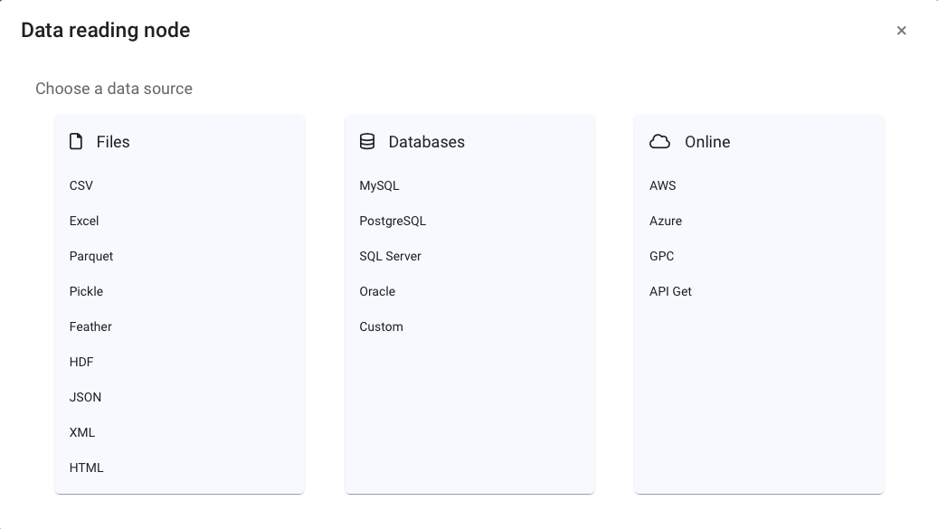
The most common options (CSV, Excel) have dedicated wizards:
Less frequently used options are initialized with base code that we then complete with the required parameters.
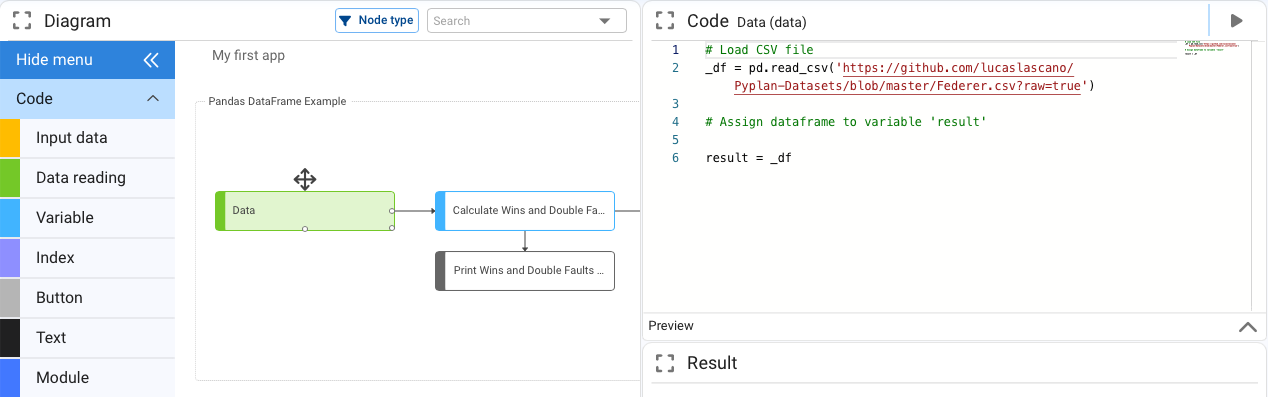
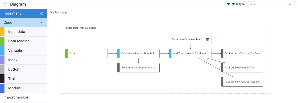
Data Manipulation and Operations
Once we have created our input nodes, the next step is to analyze and process that data using Variable nodes.
![]()
A Variable node is the most general node type: its Definition can contain any Python code. When we drag a Variable node and give it a title, it starts with result = 0.
To connect a Variable node to another node as its data source, we have two options:
- Type the node Id directly in the Definition.
- Place the cursor in the Definition and, while holding Alt, click the source node in the diagram. Pyplan automatically inserts that node's Id.
After confirming the changes, an arrow appears between the nodes showing the dependency.
Pyplan provides a set of Wizards to help us perform common data‑transformation tasks. The available wizards depend on the data structure returned by the node. Because of this, we must evaluate the node first so that Pyplan can detect the result type and determine which wizards apply.
Once the node has been executed, open the wizards by clicking the Wizards icon in the node tools bar.

Indexes
Indexes (or dimensions) define how data is structured. They act as the row and column headers of a table and describe what each value at their intersection represents. Typical examples are lists of products, regions, or time periods.
In Pyplan, we create indexes by dragging an Index node onto the influence diagram.
![]()
After assigning a title to the Index node, Pyplan opens a wizard to define its elements.
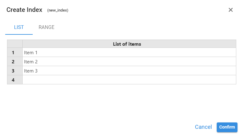
List
The List option lets us enter index elements manually:
- Type each element directly in the wizard, or
- Copy a list from an external table (e.g., Excel) and paste it.
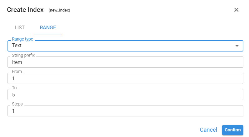
Range
The Range option generates the index automatically by defining the parameters of a range (Text, Number, or Date).
Hierarchy of Indexes
Indexes can also have hierarchies (higher levels of aggregation). For example:
- A Country index may roll up into Region or Continent.
- A Month index may roll up into Quarter, Semester, or Year.
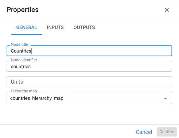
The relationship between a base index and its upper hierarchy is defined through a mapping table.
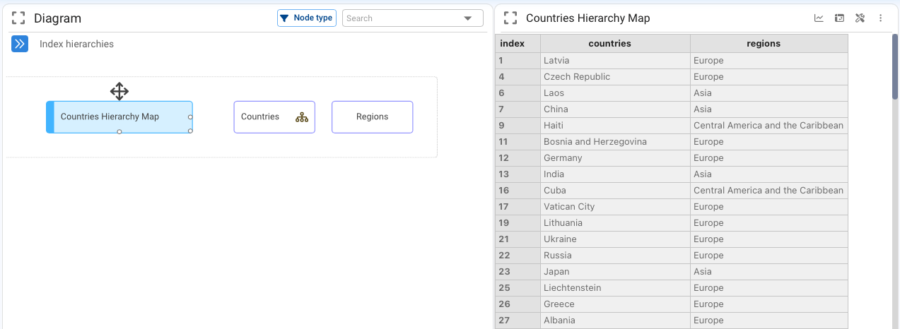
By right‑clicking the lower‑level index node and opening its Properties, we can see which table stores this correspondence with the upper hierarchy.
Any index that has a hierarchical relationship is marked with a special icon inside the node.

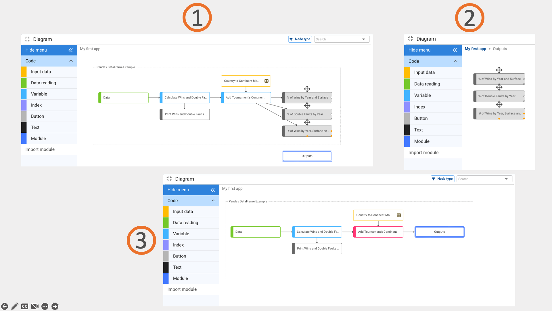
Organization of the Diagram
A good convention for readability is to keep the flow of arrows going from left to right and from top to bottom. We can also place Text nodes to group or explain sections of the diagram.
As a general rule, it is preferable not to exceed 20 nodes in a single diagram. When a diagram starts to grow beyond that, use Modules to group nodes that share a common purpose.
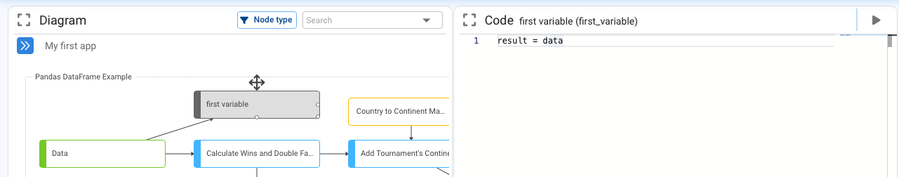
Node Coloration
Nodes are automatically colored to help us quickly understand their role:
- Most node types keep the color they have in the node palette.
- Variable nodes are the exception — their color changes according to their function in the diagram:
- Light blue — the node is part of an ongoing calculation process and has outputs in the same module.
- Gray — the node has no outputs (it behaves like a report or terminal result).
- Red — the node has outputs outside the module that contains it (cross‑module dependencies).
Node Execution
Each node can be in one of two states: Not calculated or Calculated.
When we open an application, all nodes are initially Not calculated. No calculations are performed until we explicitly run a node (double‑click, Play button, or Ctrl+Enter).
When we execute a node, Pyplan:
- Recursively walks the influence diagram upstream, checking whether all input nodes needed are already calculated.
- If any input node is not calculated, Pyplan goes one step further back and repeats the check.
- Once it reaches the application boundary or a chain of already‑calculated nodes, it evaluates the required nodes downstream in the correct order.
This mechanism ensures:
- The result of a node is always consistent, regardless of the manual order in which we previously executed other nodes.
- Only the necessary nodes are recalculated when an intermediate variable changes.
Data Structures Supported
Pyplan natively works with a set of standard data structures based on widely used Python libraries (Pandas, NumPy, xarray, etc.).
Most commonly used:
| Structure | Library | Use |
|---|---|---|
DataFrame | Pandas | Tabular data with named columns and rows |
DataArray | xarray | Named multidimensional cubes |
Array | NumPy | Unnamed multidimensional arrays |
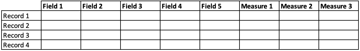
Data Tables
A table (pandas.DataFrame) is a data structure where each column represents an attribute or measure and each row represents a specific record.
Pyplan provides wizards that implement common operations on DataFrames (sorting, filtering, aggregation, joins, etc.). Any additional transformation can be implemented directly in Python using the full Pandas API.
Assisted Operations with Tables
When a node returns a DataFrame, Pyplan automatically enables a set of wizards for that node.
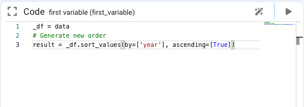
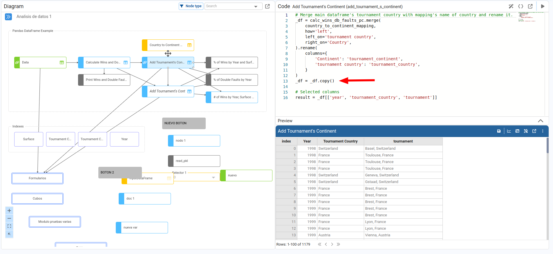
For example, choosing Sort by Year will:
- Apply the requested operation to the DataFrame.
- Update the node result accordingly.
- Modify the node Definition to include the corresponding Pandas code.
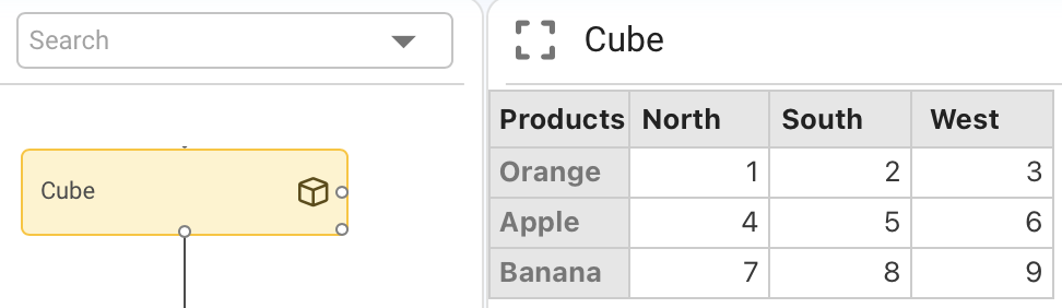
Data Cubes
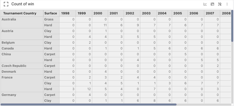
A data cube is natively supported in Pyplan as xarray.DataArray. A named data cube stores values indexed by n named dimensions.
For example, a "Count of Win" cube indexed by Tournament Country, Surface, and Year stores one value per combination.
Data cubes in Pyplan can be created by:
- Transforming tables (
DataFrame) into cubes. - Direct manual inputs (Input Cube or Input Table nodes).
- Performing operations between existing cubes.
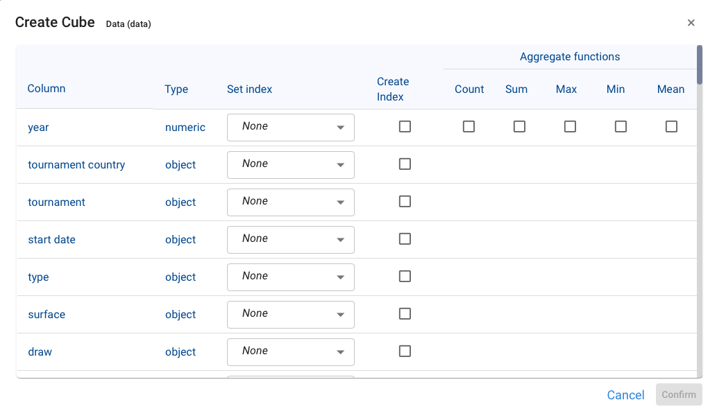
Creating a Cube from a Data Table
- Click the arrow to the right of the node that returns the table.
- In the context menu, choose Transform → Create cube.
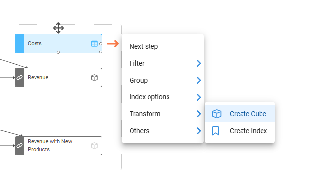
Pyplan opens a dialog showing, for each column of the DataFrame, its name, data type, associated Index (if one already exists), and the aggregation function to apply.
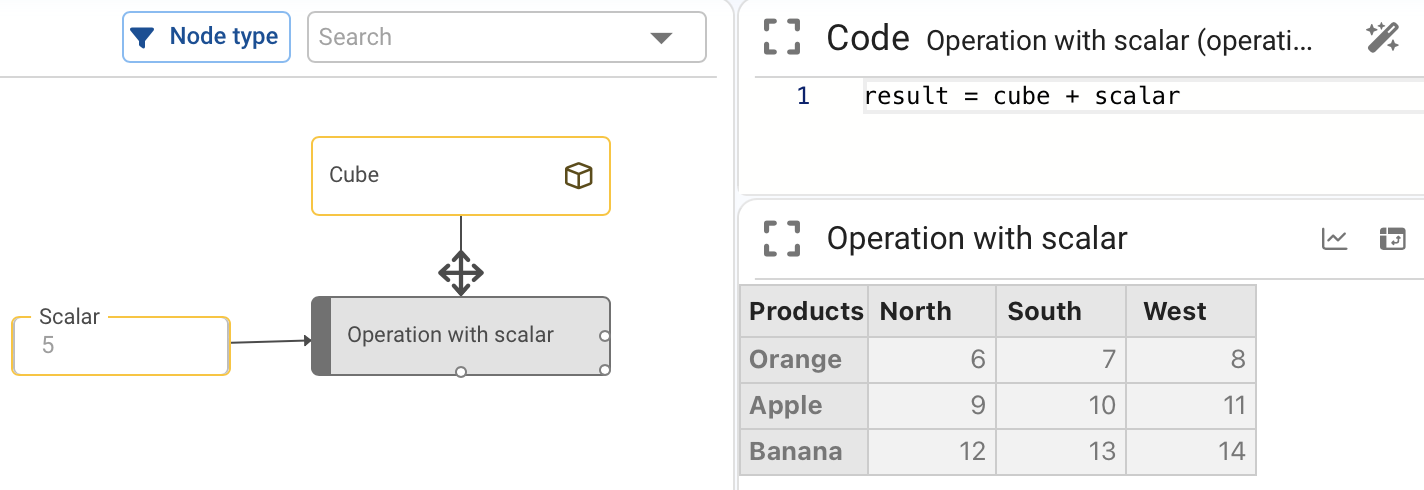
Operations with Data Cubes
When a node returns a DataArray, Pyplan enables a set of cube wizards. In addition, cubes support element‑wise mathematical operations between them.
Operations between a scalar and a cube:
If scalar equals 5, then cube + scalar adds 5 to every element of the cube.
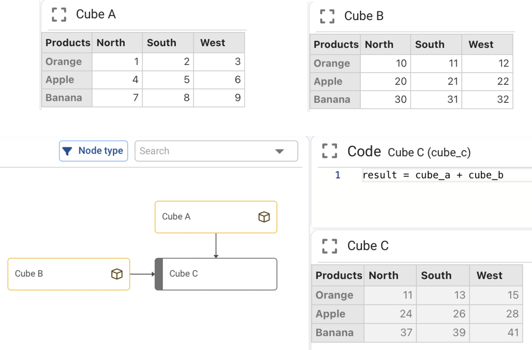
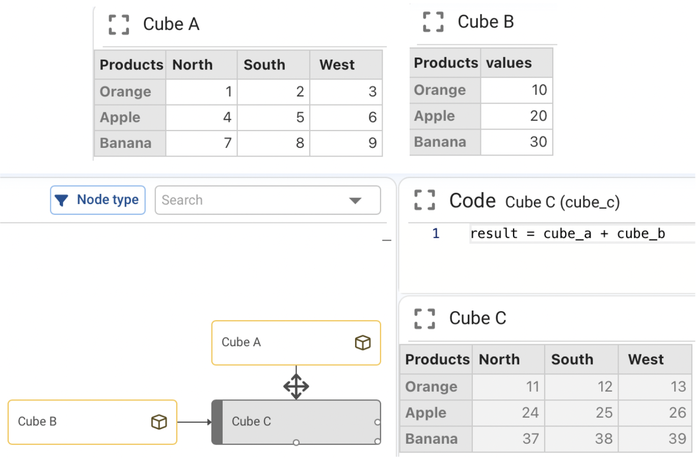
Operations between two cubes of equal dimensions:
The operation is performed cell by cell.
result = cube_a + cube_b
Operations between two cubes of different dimensions (broadcasting):
When operating on cubes with different dimensions, the missing dimension is broadcast. For example, if cube_a has dimensions [Product, Region, Year] and cube_b has [Product, Year]:
result = cube_a + cube_b
cube_b is broadcast across the Region dimension — for each (Product, Year) pair, the same value from cube_b is added to all regions in cube_a.
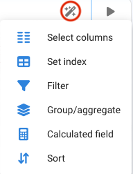
Wizards to Manipulate DataFrame Nodes
Pyplan includes a set of wizards that help us transform pandas.DataFrame results without writing all the code manually.
To open these wizards:
- Execute the node that returns the DataFrame.
- Open the node menu (right‑click or menu icon on the node).
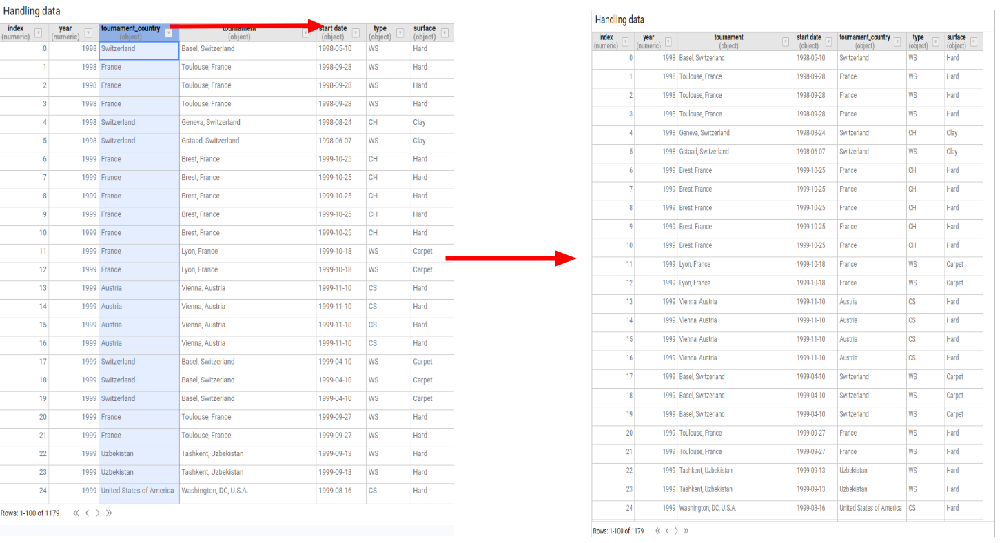
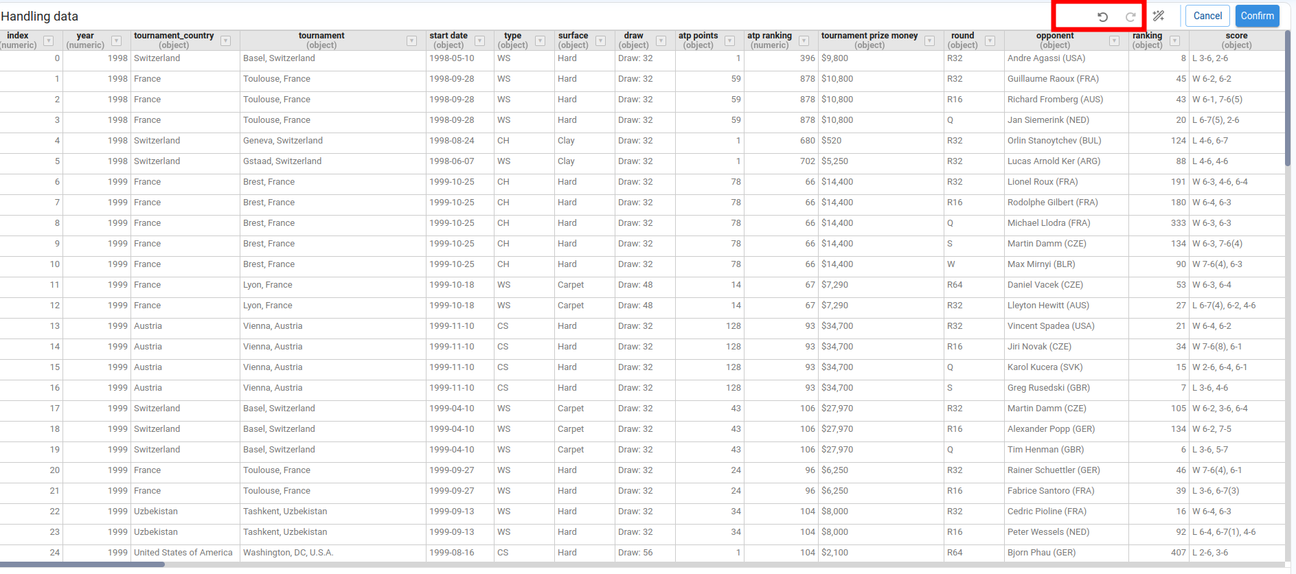
- Select Handling data.
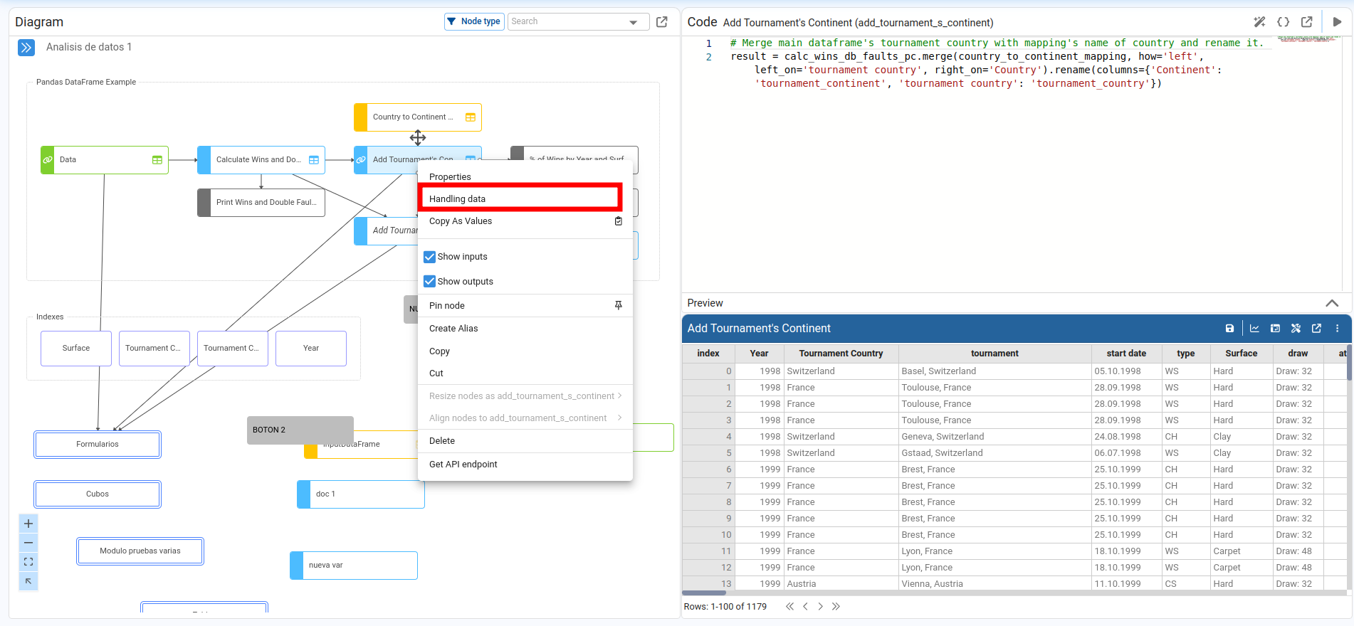
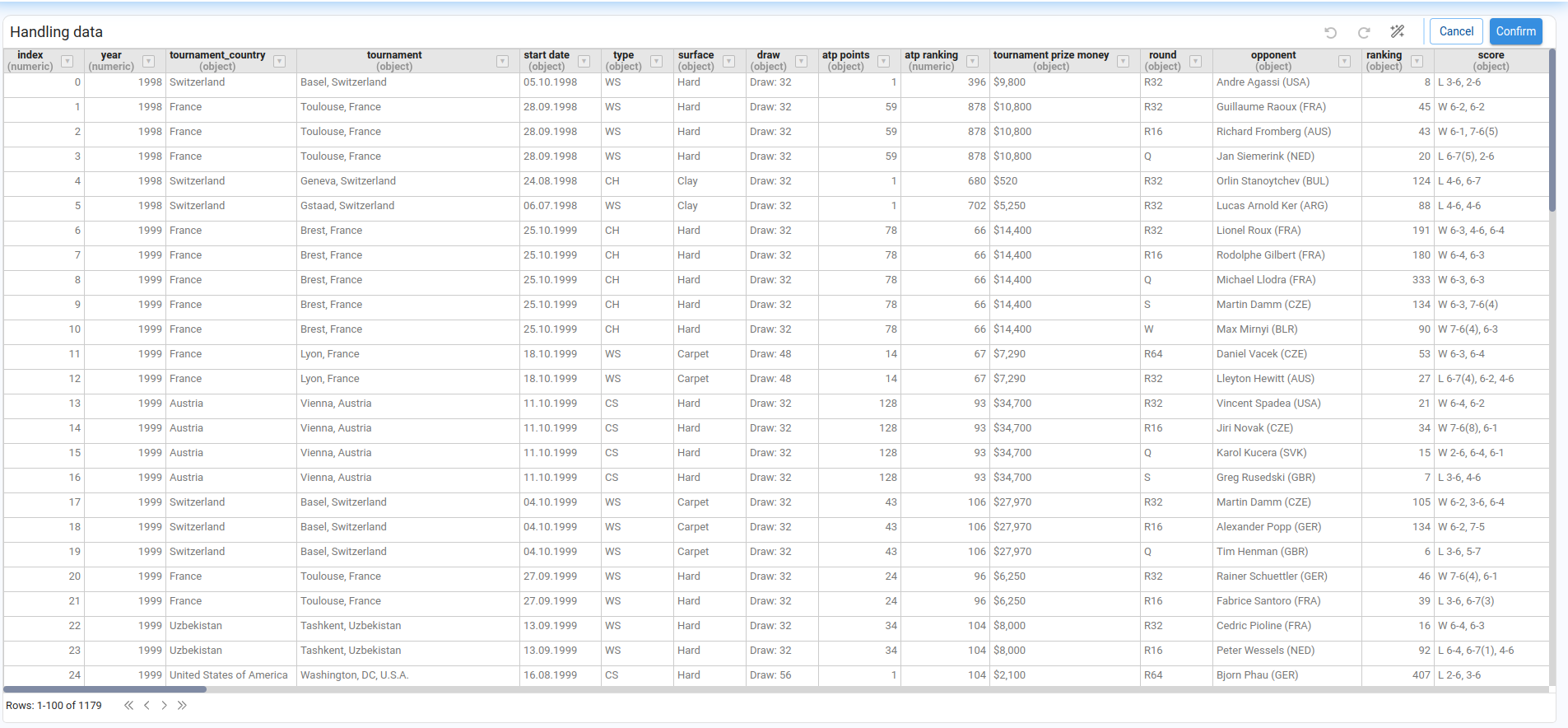
A widget opens showing the node result in a paginated table. Column headers display both the column name and its data type.
The available wizards are grouped into two categories:
-
Wizards that affect the entire DataFrame.
-
Wizards that affect only a single column.
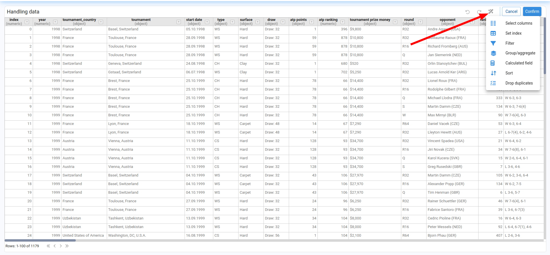
Wizards That Impact the Entire DataFrame
Select Columns
Lists all columns with their data type and an indicator showing whether each column is an index. We select the columns we want to keep and confirm.
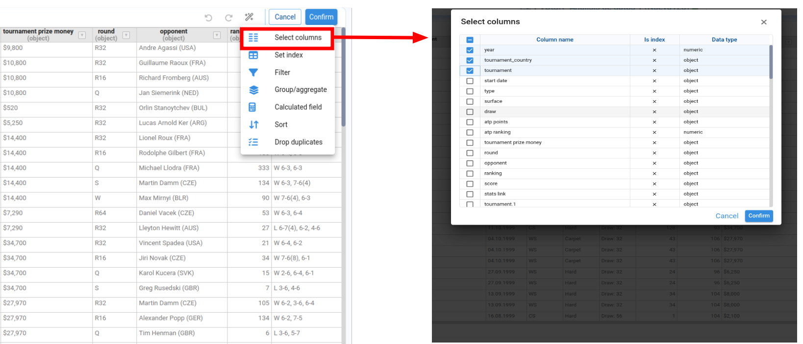
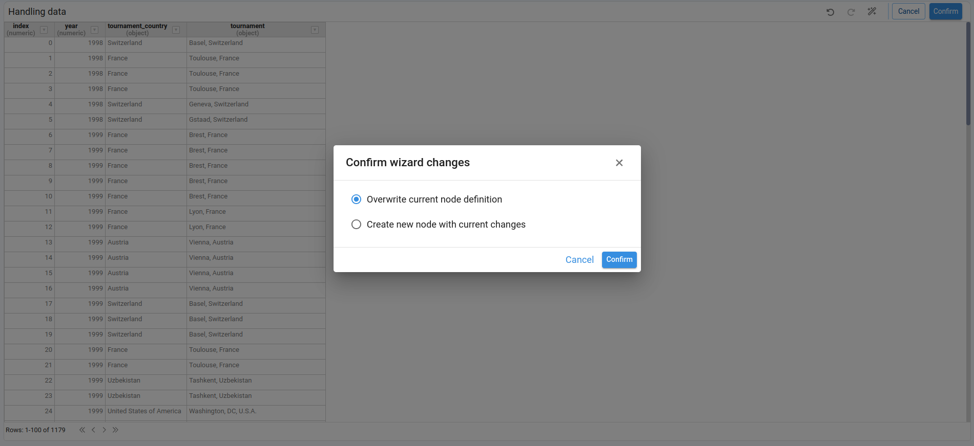
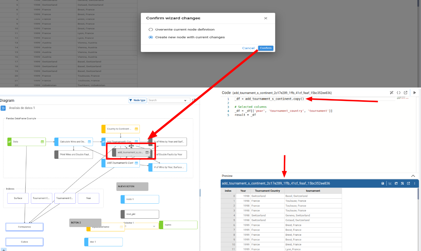
When we confirm, we can choose to:
- Overwrite current node definition, or
- Create a new node with the transformed DataFrame.
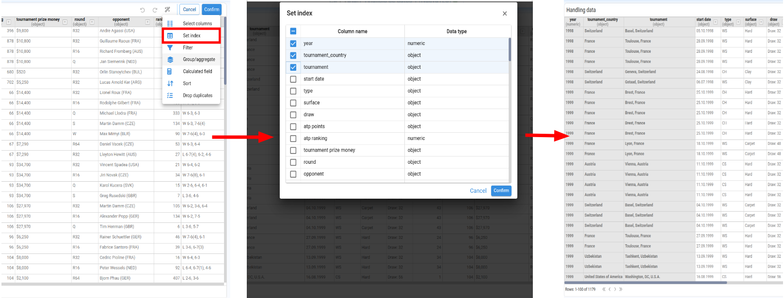
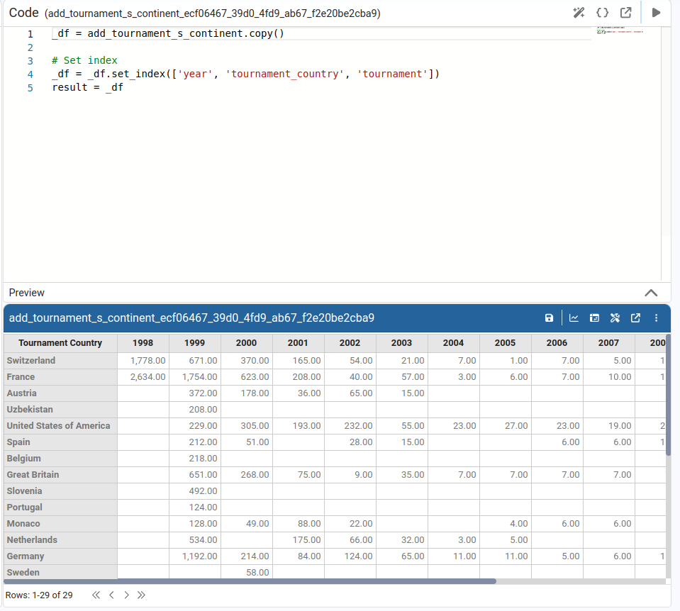
Select Index
Lets us choose one or more columns to act as indexes of the DataFrame.
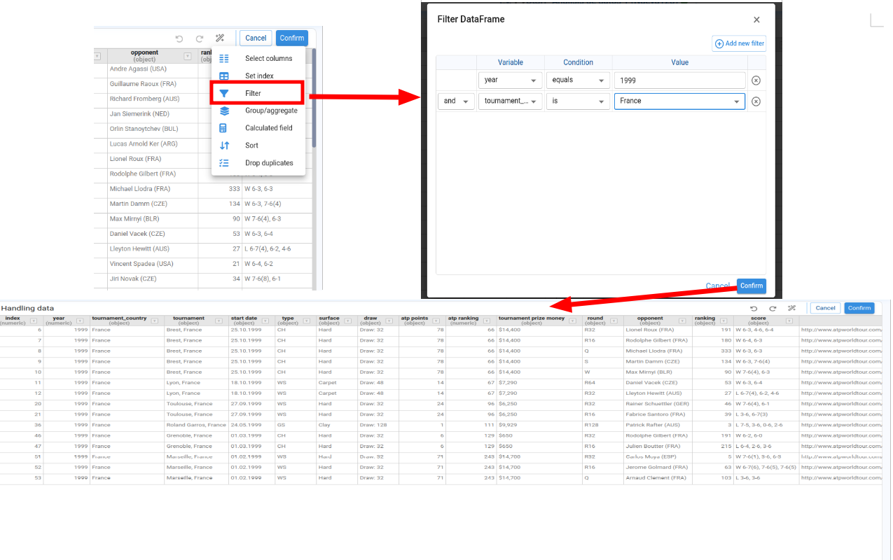
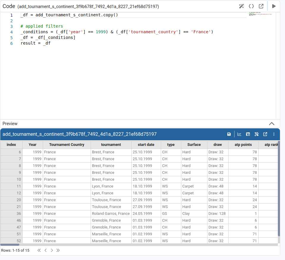
Filter Rows
Allows us to apply one or more filter conditions to the DataFrame. Filters are combined using AND or OR.
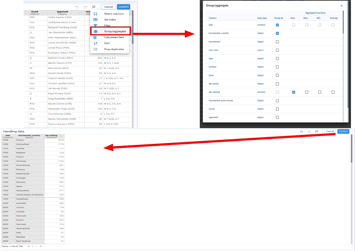
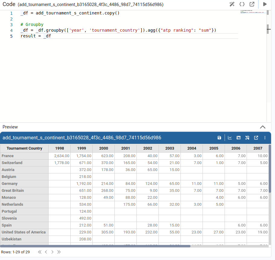
Group / Aggregate
Used to perform aggregations. We choose the grouping columns and the aggregation functions (sum, mean, count, etc.) for the numeric columns.
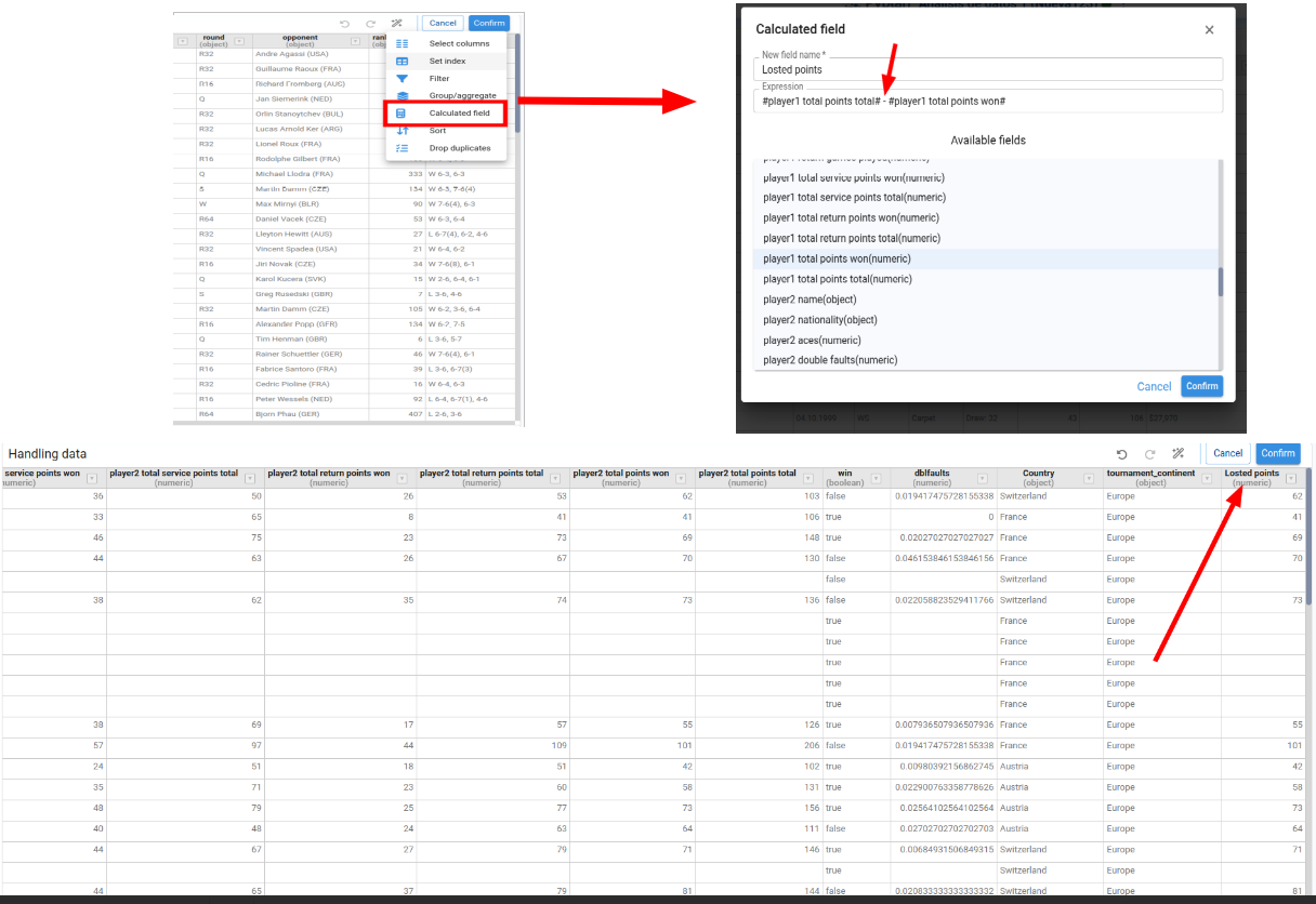
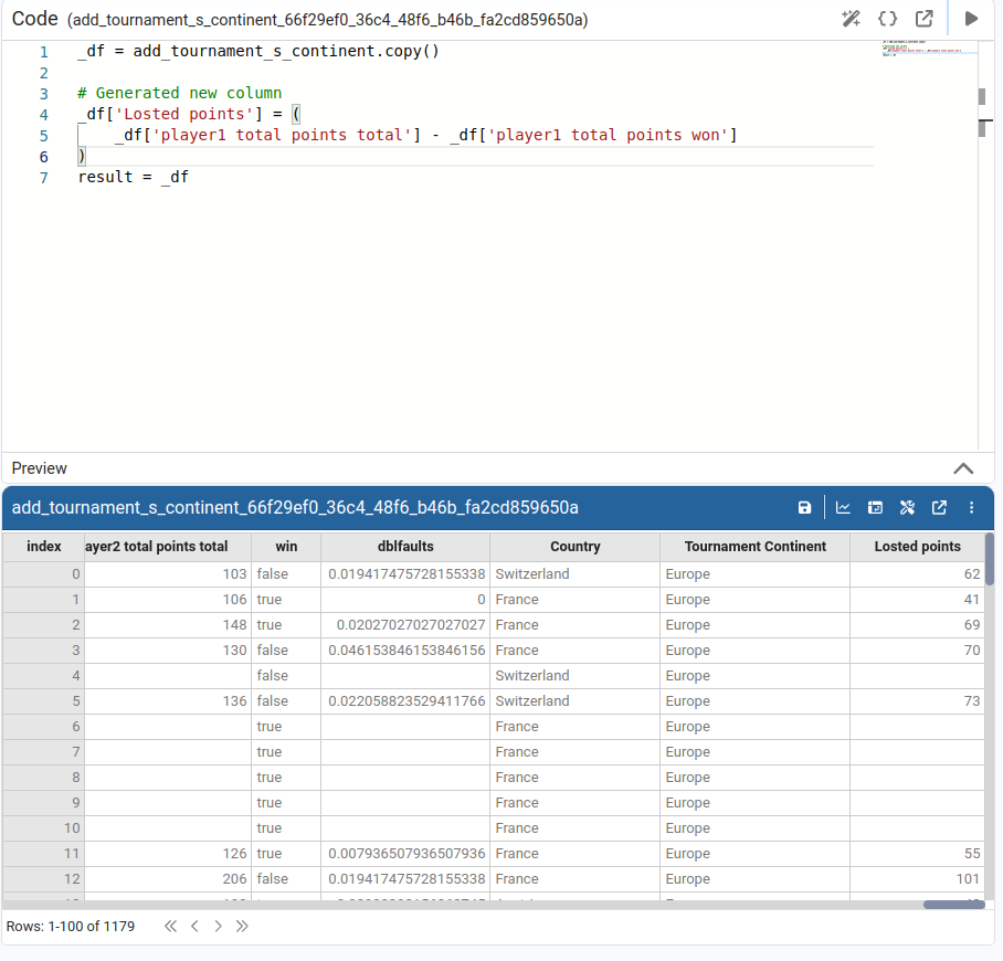
Add Calculated Field
Lets us add a new calculated column to the DataFrame by specifying the new column name and defining the calculation as an expression combining existing columns.
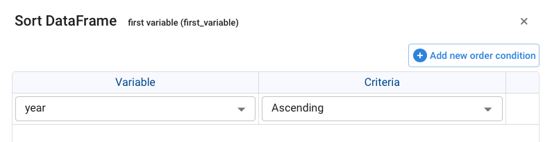
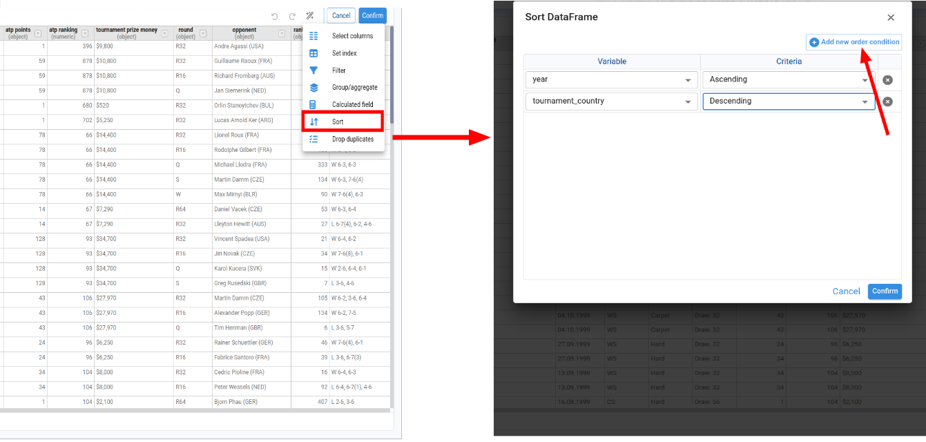
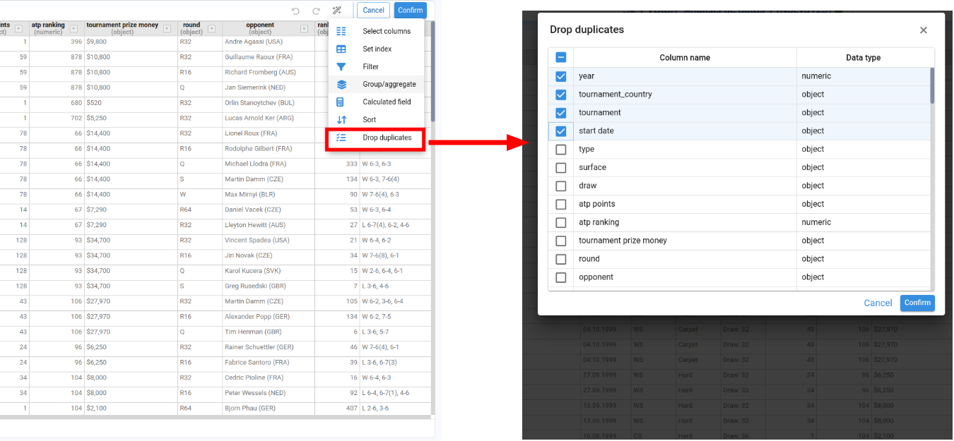
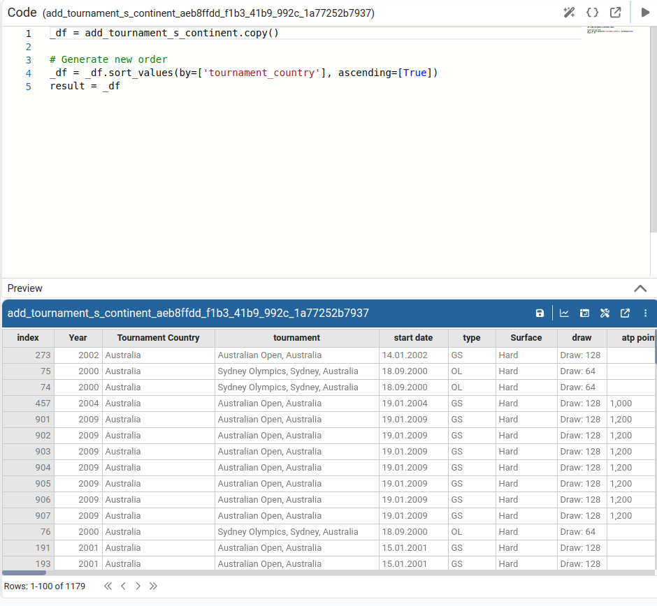
Sort DataFrame
Sorts the table by one or more columns, choosing ascending or descending order for each.
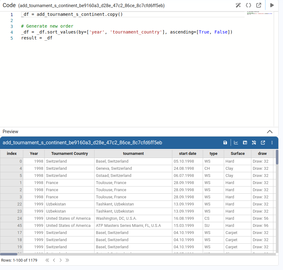
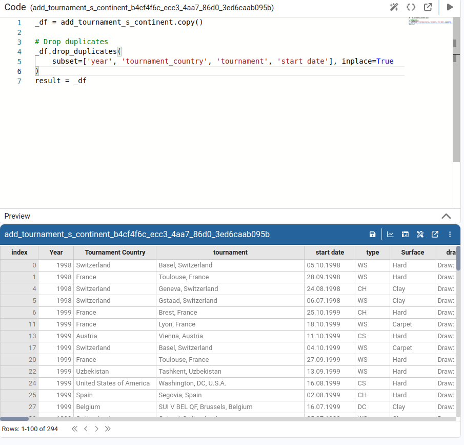
Drop Duplicates
Lists all columns and lets us choose the subset of columns to consider when removing duplicate rows.
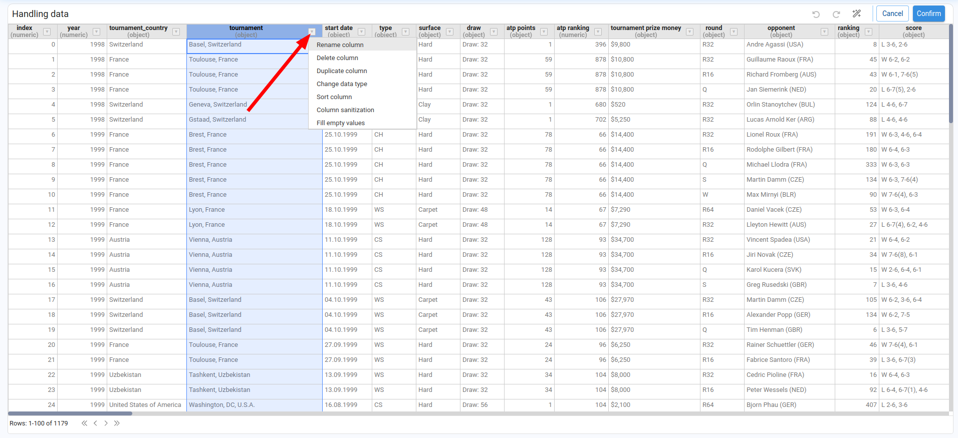
Wizards That Impact at the Column Level
These wizards operate only on the selected column. They are available from the table header of each column.
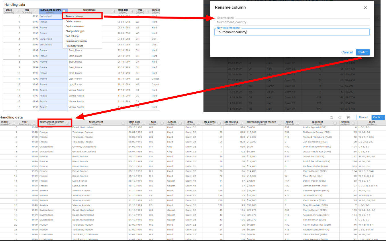
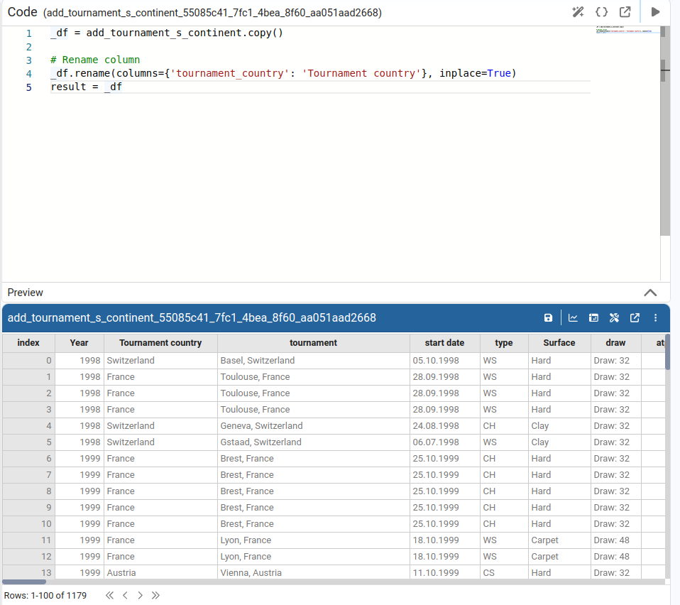
Rename Column
Lets us enter a new name for the selected column.
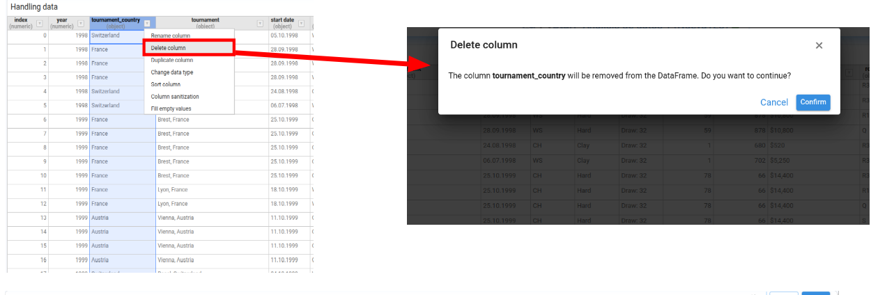
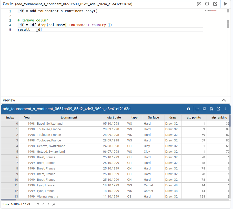
Delete Column
Removes the selected column from the DataFrame.
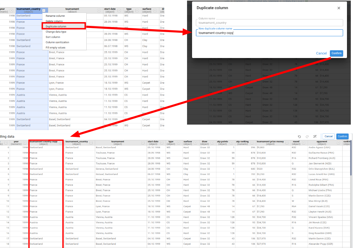
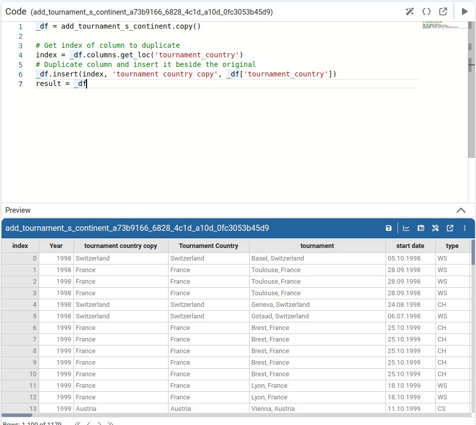
Duplicate Column
Creates a copy of the selected column with a new name.
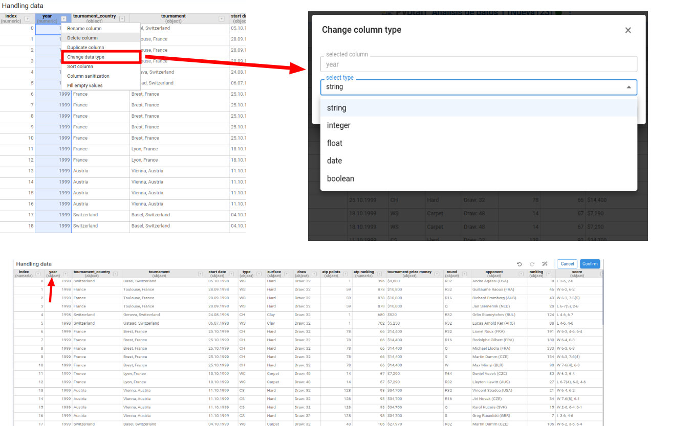
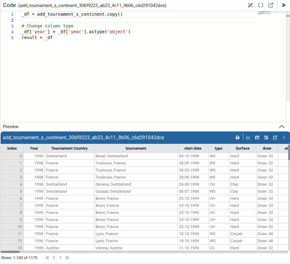
Change Data Type
Changes the data type of the selected column. Available target types: string, integer, float, date, boolean. When we choose date, we can also specify a date format.
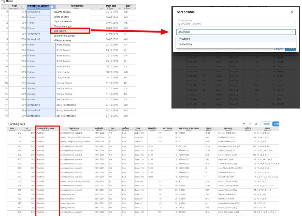
Sort Column
A simplified sort that only changes the order of the selected column (ascending or descending).
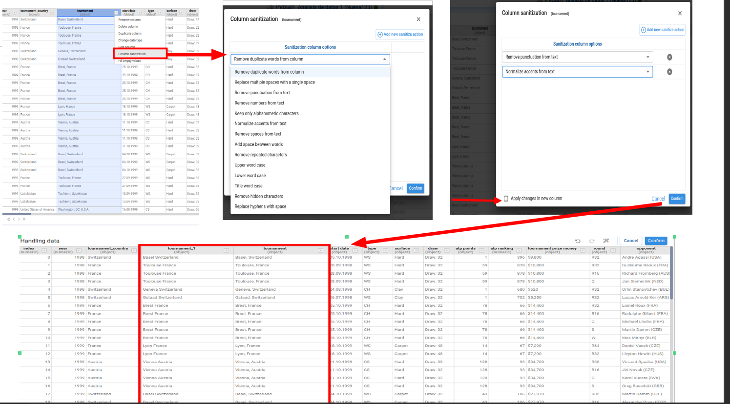
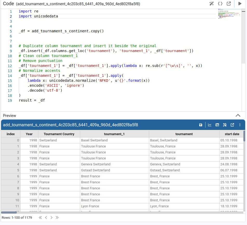
Sanitize Column
Applies one or more clean‑up operations to the entire column (trimming spaces, changing case, replacing characters). We can choose whether to apply the changes in a new column or overwrite the current column.
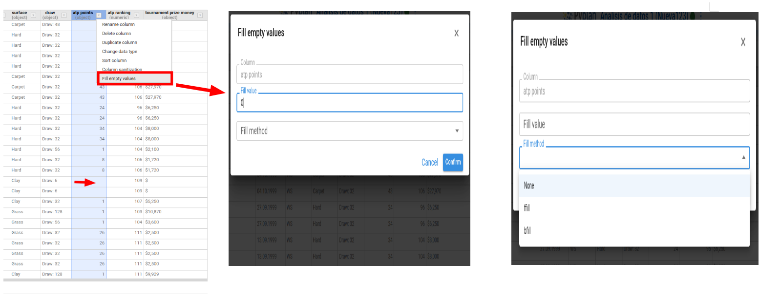
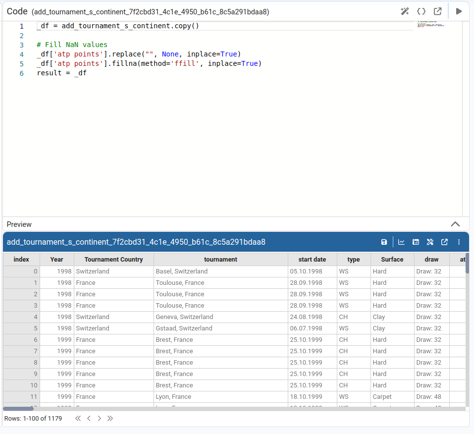
Fill Empty Values
Fills missing or empty values in the column with a default value. Options:
- Fill value — literal replacement (e.g.,
0,'N/A'). - Forward fill (
ffill) — use the last non‑null value above. - Backward fill (
bfill) — use the next non‑null value below.
Additional Features
Pyplan keeps an internal history of changes so we can Undo and Redo transformations.
We can also reorder columns by selecting one or more columns and dragging them to the desired position in the table. This reordering is immediately reflected in the node Definition.